
If your mission is work management, IBM i is the best starship in the fleet. Routing certain types of work into subsystems and memory pools, separating dissimilar work, and giving jobs the appropriate CPU time—this is work management the Windows world can only dream about.
Unfortunately, they also make IBM i performance tuning difficult to command. Get a head start with 3 settings that can put IBM i work in warp drive.
What is Work Management?
Work management is work entering the computer system and the resources it uses. What makes this topics so important for IBM i shops is the flexibility that the OS gives you.
All jobs on the system can be controlled as to where they run and the resources they use depending upon the needs of the business, but many commanders become overwhelmed by the options:
- Why does the interactive session run the subsystem that it does?
- Should batch jobs run in the *BASE memory pool?
- Why doesn’t that subsystem start up automatically when you IPL your system?
- Why is the system memory pool 1 the size that it is?
- What is a routing entry?
This article may be a refresher for some, but many operators have inherited the i and are unfamiliar with IBM i work management techniques. By supporting multiple types of workloads with customized environments, IBM i comes naturally equipped to put your jobs in warp drive. For example, here's how work management affects batch jobs:
Step 1—Know Your Enterprise
Your batch subsystem description contains many attributes. Subsystems should be configured to start up automatically in the IPL program defined in the system value QSTRUPPGM.
Funny thing is—the order in which the subsystems start is the order in which memory pools are allocated on the system—except for system pool 1 (*MACHINE) and pool 2 (*BASE).
By default, your operating system runs the *MACHINE pool with all unallocated memory in *BASE. All other memory pools pull memory from *BASE.
In this training system (Figure 1), the *INTERACT pool is assigned as system pool 3 because the QINTER subsystem was started first, followed by a subsystem containing *SHRPOOL1, and finally the QSPL subsystem.
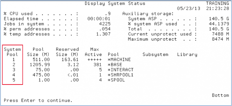
Figure 1 – DSPSYSSSTS command showing system memory pools
IBM i creates pools and allocates memory to them based on the “Pool Definition” on the subsystem description (Figure 2). Some memory pools can be shared such as *SHRPOOL1 and some can be private pools.
Don’t get yourself confused just yet, the amount of memory and max active (activity levels) are a discussion for another day.
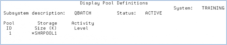
Figure 2 – DSPSBSD option 2 Pool Definitions
Step 2—Entering the System
Job are initiated (or enter the system) in different ways.
Batch jobs are initiated by the SBMJOB command. There are many parameters on the SBMJOB command and we could devote an entire article just to that topic.
For this discussion, the JOBQ parameter is critical because it routes your job into a work management tool called a job queue where the number of jobs that go active can be controlled (single threaded, 10 at a time, etc.) but also sets up the job to run in a particular memory pool via the “Routing data” (Figure 3).
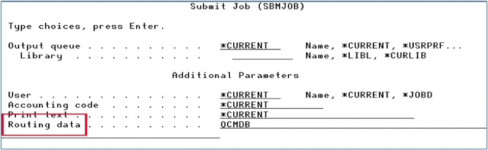
Figure 3 – SBMJOB command and the routing data parameter
This routing data is compared to the “Routing entry” in the subsystem description (Figures 4 and 5). The routing data will either match one of the entries or it will fall through to the *ANY compare value.
In our QBATCH subsystem the *ANY compare value specifically says to route work into the subsystem pool 1, which is defined as *SHRPOOL1.
*SHRPOOL1 is also known as system pool 4 in figure 1 —again due to the order in which the subsystems were started. So we’ve now discovered that *SHRPOOL1 was defined on the QBATCH subsystem and that subsystem was started next in line after QINTER. Whew!
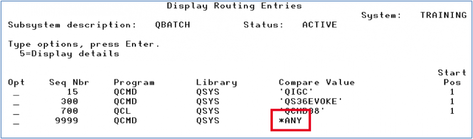
Figure 4 – DSPSBSD option 7 Routing Entries
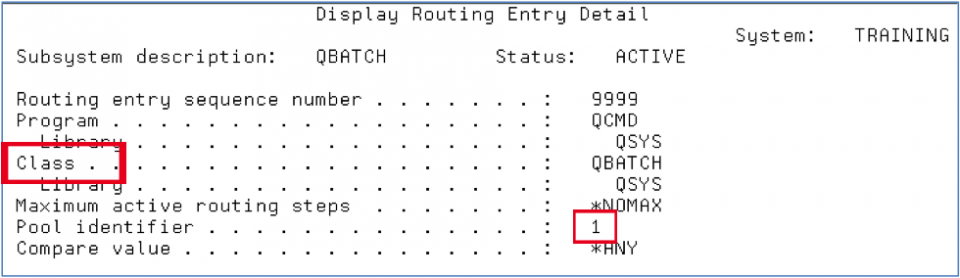
Figure 5 – DSPSBSD option 7 Routing Table Entry for *ANY
Step 3—Speeds and Feeds
Not only does the routing entry determine the memory pool that the work is allocated but it also determines the CPU priority and time slice that the work will receive. Figure 5 shows that the batch job using this routing entry will run using the class QSYS/QBATCH.
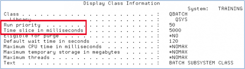
Figure 6 – DSPCLS command
Reviewing the QBATCH class reveals that this batch job gets a Run Priority of 50 and a time slice of 5000 milliseconds (5 seconds). This is a lower run priority than interactive work which runs at a 20 but a longer time slice than the typical 2000 milliseconds for interactive jobs.
The theory is that interactive users need priority when they press the enter key but typically don’t need as much CPU time to complete the request, as opposed to a batch job processing thousands or millions of records.
What happens at the end of this time slice? Either the job completes or it gets in line and waits for another opportunity for CPU time along with all the other work on the system.
All tasks running on the system are competing for processor time and their turn to use it. In addition, the system performance tuner, or Robot Autotune, is adjusting the amount of memory in the system pools and the number of jobs or threads that can actively compete for the processor.
This is part of the tuning and queuing process that the operating system handles automatically for you and takes all the run priorities, job wait times, memory, and activity levels into account.
We’ll be exploring more work management, performance tuning and other advanced systems management topics, including PowerHA and IASP (independent auxiliary storage pools) in the next few months.
Until then, live long and prosper.
Get Started
Ready to identify issues and fix them before end users feel the impact? See how Fortra solutions for proactive performance and application monitoring keeps downtime out of the picture.